Mapas Temáticos usando o R - Parte 2.

Como continuação do post Mapas Temáticos usando o R, mostraremos aqui como é possível unir informações pontuais (Point Process) e dados regionais (Lattice Data) além de unir esses dados com o Google maps.

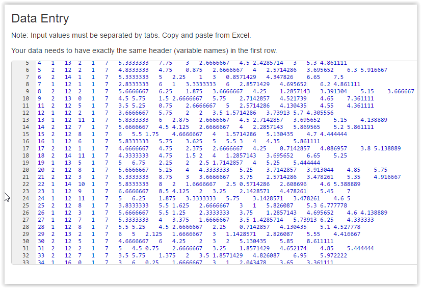
O primeiro passo é a obtenção da malha (shapefile) e dos dados (DadosMapa.csv) para o processo de georeferenciamento.

O primeiro passo é invocar as bibliotecas necessárias bem como definir o Working Directory no qual o arquivo DadosMapa.csv está e também a pasta Shapes

?

1 2 3 4 5 6 7 8 9 10 11 12 13 14 15

#Limpa o Working Directory rm(list=ls()) #Define working directory setwd("C:\\Blog\\ExemploMapas") #Invoca os pacotes necessários library(RColorBrewer) library(maptools) library(rgdal) library(rgeos) library(RgoogleMaps) library(sp) library(spdep) library(ggmap) library(plyr) library(Hmisc)

Em seguida, importamos para o R os dados e a malha de interesse:

?

1 2 3 4

#Importa os dados dados<-read.csv("DadosMapa.csv") #Lê os shapefiles que estão na pasta Shapes dentro do working directory sfn <- readOGR("Shapes","11MUE250GC_SIR",verbose = FALSE)

Uma vez lidos os dados e malhas, é preciso saber qual a região devemos importar do GoogleMaps, para isso fazemos:

?

1 2 3 4 5 6 7 8 9 10 11 12 13 14 15 16 17 18

#Bounding box a ser utilizada no ggmap b <- bbox(sfn) #Cria uma variável ID para o georeferenciamento sfn@data$id <- rownames(sfn@data) #Define a projeção (Shapefile) sfn <- spTransform(sfn, CRS("+proj=longlat +datum=WGS84")) #Cria um SpatialPointsDataFrame com as latitudes e longitudes dos dados spdf <- SpatialPointsDataFrame(coords=dados[,c("Longitude","Latitude")], data=dados) #Define a projeção para os pontos proj4string(spdf) <-CRS("+proj=longlat +datum=WGS84 +no_defs +ellps=WGS84 +towgs84=0,0,0") #Trasnforma o objeto espacial em um objeto que pode ser lido pelo ggplot2 sfn.df <- fortify(sfn, region="CD_GEOCMU") #Substring a variável ID para ficar com 6 dígitos (ignora o dígito verificador) sfn.df$V007<-substr(sfn.df$id,1,6) #Left Join do CSV com o Shapefile sfn.df<-merge(sfn.df,dados,by="V007",all.x=T) #Ordena os dados sfn.df<-sfn.df[order(sfn.df$order), ]

Finalmente, após a união dos dados com o Shapefile podemos construir o mapa. Para isso passamos como argumento do ggmap a bounding box obtida nos passos anteriores e definimos também as cores, escalas, títulos do mapa:

?

1 2 3 4 5 6 7 8 9 10 11 12 13 14 15 16 17 18 19 20

#Aumenta ou diminui a Bounding Box (aumenta em 1%) bbox <- ggmap::make_bbox(sfn.df$long, sfn.df$lat, f = 0.1) #Escolhe as cores myPalette <- colorRampPalette(rev(brewer.pal(11, "Spectral"))) #Obtêm o mapa do Google Maps (Existem outras possibilidades...) map <- get_map(location=bbox, source='google', maptype = 'terrain', color='bw') #Constrói o mapa: map <- ggmap(map, base_layer=ggplot(data=sfn.df, aes(x=long, y=lat)),              extent = "normal", maprange=FALSE) map <- map + geom_polygon(data=sfn.df,aes(x = long, y = lat, group = group, fill=Valor), alpha = .6)  map <- map +   geom_path(aes(x = long, y = lat, group = group),                          data = sfn.df, colour = "grey50", alpha = .7, size = .4, linetype=2)  map <- map + coord_equal() map <- map + scale_fill_gradientn(colours = myPalette(4)) map<-map+  geom_point(aes(x=Longitude, y=Latitude),color="black", size=1,                       alpha = 0.70,                       data=spdf@data) map<-map +  ggtitle("Postos SINE") +  labs(x="Longitude",y="Latitude") #Plota o mapa plot(map)

Pode-se ainda definir outras bases para o shapefile, alguns exemplos são apresentados a seguir:

?

1 2 3 4 5 6 7 8 9 10 11

##Pode-se trocar o código: map <- get_map(location=bbox, source='google', maptype = 'terrain', color='bw') ##Do bloco anterior, por algum desses outros: #map <- get_map(location=bbox, source='osm', color='bw')) #map <- get_map(location=bbox, source='stamen', color='watercolor')) #map <- get_map(location=bbox, source='stamen', color='toner')) #map <- get_map(location=bbox, source='stamen', color='terrain')) #map <- get_map(location = bbox, source = 'google', maptype = 'terrain') #map <- get_map(location = bbox, source = 'google', maptype = 'satellite') #map <- get_map(location = bbox, source = 'google', maptype = 'roadmap') #map <- get_map(location = bbox, source = 'google', maptype = 'hybrid')

Executando R online com R-FIDDLE.COM

www.R-fiddle.org é um ambiente livre e poderoso para escrever, executar e compartilhar códigos escritos em R.

Esse ambiente ainda oferece a opção de instalar pacotes. Em suma, uma ótima ferramenta para aqueles que querem ensinar ou aprender R sem a necessidade de instalar nenhum arquivo adicional em sua máquina.

Ao entrar no site www.R-fiddle.org observa-se a seguinte tela:

Na parte de baixo os códigos em R são inseridos na forma de Console, por exemplo:

Já na região em branco os códigos são inseridos na forma de Script. Após inseridos os códigos de interesse, basta clicar em Run Code. Os pacotes são invocados normalmente. Ou seja, uma ótima oportunidade para aprender R e compartilhar códigos de maneira simples e direta!!

Edição Colaborativa em Latex.

Overleaf é um sistema de escrita e publicação colaborativa em Latex que torna todo o processo de produção de trabalhos acadêmicos muito mais rápido para ambos os autores e editores. Overleaf é um serviço gratuito que permite criar, editar e partilhar as suas ideias científicas facilmente online usando Latex, uma ferramenta abrangente e poderosa para a escrita científica.

Uma das vantagens Overleaf é o fato de que essa plataforma apresenta uma diversidade de possíveis templates, facilitando assim a escrita em Latex:

Adtei um modelo da USP para a Universidade de Brasília no Overleaf. Para acessá-lo, clique aqui!

Equações Estruturais usando lavaan.shiny.

O pacote lavaan.shiny é uma ótima ferramenta para quem possui dificuldades com a programação em R, mas deseja fazer análises complexas envolvendo Equações Estruturais.

?

1 2 3 4 5 6 7 8 9 10

#Limpa o Workspace rm(list=ls()) #Instalçao do pacote lavaan.shiny install.packages("lavaan.shiny") #Instalçao do pacote para gráficos install.packages("DiagrammeR") #Invoca a biblioteca library(lavaan.shiny) #Abre o shiny do lavaan lavaan.shiny()

Após a execução desse código, o R apresenta uma tela mais amigável para o desenvolvimento dos modelos de Equações Estruturais, a seguir um exemplo de especificação do modelo:

O próprio lavaan.shiny já apresenta um exemplo pronto de um modelo de Análise Fatorial Confirmatória baseado no trabalho de Holzinger, K. J., & Swineford, F. (1939). A study in factor analysis: the stability of a bi-factor solution. Supplementary Educational Monographs.

Para realizar uma análise prática, o primeiro passo é a inserção do banco de dados de interesse. No final da página do lavaan.shiny você deve copiar e colocar os dados. Você pode fazer isso copiando e colando direto do Excel:

Ao continuar descendo na página há ainda outros resultados, como estatísticas descritivas, correlações, estimativas dos parâmetros e também o gráfico de caminhos:

O pacote lavaan.shiny é uma ótima opção para aqueles que desejam trabalhar com modelos como Análise Fatorial Confirmatória e Equações Estruturais sem a necessidade de programação.

A única programação necessária é a instalação do pacote e execução da função lavaan.shiny() todo o resto ocorre em um navegador na máquina do usuário.

Mapas Temáticos usando o R.

Mapas Temáticos são muito utilizados na etapa de Análise Espacial Exploratória, a qual tem por principal objetivo apresentar visualmente a existência de algum possível padrão espacial.

O objetivo desse post é apresentar como é possível construir Mapas Temáticos usando o R.

O primeiro passo é a obtenção de uma malha digital. Usualmente, uma malha digital é um conjunto de pelo menos três arquivos com o mesmo nome, mas extensões diferentes (*.dbf,*.shx,*.shp). Essa malha nada mais é do que as delimitações geográficas do mapa de interesse. Por exemplo, suponha que desejamos construir um Mapas Temático para os municípios brasileiros, precisamos então da malha municipal.

O principal repositório de malhas digitais no Brasil é do IBGE. Nesse link (ftp://geoftp.ibge.gov.br/malhas_digitais/) podemos obter as mais diversas malhas digitais. Nesse exercício trabalharemos com a malha municipal de 2005.

O código a seguir lê a malha digital (55mu2500pc) e cria uma outra malha somente com o contorno das Unidades da Federação:

?

1 2 3 4 5 6 7 8 9 10 11 12

#Limpa o Workspace rm(list=ls()) #Chama a biblioteca library(ggplot2) library(rgdal) library(plyr) library(rgeos) #Carrega o objeto SpatialPolygon br <- readOGR(dsn = ".", "55mu2500pc", verbose=FALSE) #Faz o dissolve para as UF's UF <- gUnaryUnion(br, id = br@data$UF) UF <- fortify(UF, region="UF")

Em seguida, precisamos obter um conjunto de dados que desejamos plotar no mapa. Esse conjunto deve possuir pelo menos uma variável identificada pelo Código do Município também presente na malha 55mu2500pc. Vamos usar como exercício os dados do IpeaData (basta pesquisar no campo Regional pelo tema "Número de homicídios" ou baixe o arquivo aqui.).

?

1 2 3 4 5 6 7 8 9 10 11 12 13 14 15 16 17 18 19 20 21 22 23 24 25 26

#Lê os dados all_content <- readLines("ipeadata.csv") #Pula o nome das colunas skip_first = all_content[-1] #Lê os dados indice<- read.csv2(textConnection(skip_first), header = TRUE, stringsAsFactors = FALSE) #Transforma o NA em zero indice[is.na(indice)] <- 0 #Corrige o nome dos municípios enconding indice[,3]<-iconv(indice[,3], "UTF-8", "LATIN2") indice<-indice[,-9] colnames(indice)<-c("Sigla","Codigo","Mun","C2005","C2006","C2007","C2008","C2009")   #Renomeia as colunas indice$GEOCODIGO<-as.character(indice$Codigo) #Indice de Criminalodade em 2005 indice$Indice<-indice$C2005/sum(indice$C2005) #Cria as categorias indice$Categorias1<-cut(indice$Indice,c(0, 0.25,0.50,0.75,1),                      labels=c('<0.25','0.25|-0.50','0.50|-0.75','>=0.75')) #Categorias por quartil breaks<-c(quantile(indice$Indice, probs = seq(0, 1, by = 0.25))) breaks[1]<-breaks[2]-1e-5 indice$Categorias2<-cut(indice$Indice, breaks=breaks,   labels=c("1º Quartil","2º Quartil","3º Quartil","4º Quartil"),   include.lowest=TRUE)

Agora é preciso unir os dados com a malha:

?

1 2 3 4 5 6 7

#Faz o merge com os dados br@data$id <- rownames(br@data) #Caso o código tenha apenas 6 dígitos: br@data$IBGE<-substr(br@data$GEOCODIGO,1,6) br@data   <- join(br@data, indice, by="GEOCODIGO") #Cria o objeto para ggplot2 br.df <- fortify(br) br.df <- join(br.df,br@data, by="id")

Em seguida fazemos o mapa:

?

1 2 3 4 5 6 7 8 9

#Define as cores do mapa library(RColorBrewer) myPalette <- colorRampPalette(brewer.pal(11, "Spectral")) #Faz o mapa Map <- ggplot(br.df, aes(long, lat)) + geom_polygon(aes(group = group, fill = Categorias2)) +   coord_equal() + labs(x = "Longitude", y = "Latitude", fill = "Criminalidade\nRegional") +   ggtitle("Índice:\n Criminalidade Regional") +   geom_polygon(data=UF, aes(group=group), alpha=1,colour="black", fill=NA, size=0.5) Map

Caso deseje fazer o mapa com o valor numérico também é possível usar o argumento scale_fill_gradientn:

?

1 2 3 4 5 6 7

#Faz o mapa Map2 <- ggplot(br.df, aes(long, lat)) + geom_polygon(aes(group = group, fill = Indice)) +   coord_equal() + labs(x = "Longitude", y = "Latitude", fill = "Criminalidade\nRegional") +   ggtitle("Índice:\n Criminalidade Regional") +   scale_fill_gradientn(colours = myPalette(4))+   geom_polygon(data=UF, aes(group=group), alpha=1,colour="black", fill=NA, size=0.5) Map2

Usando a Biblioteca libSVM no R - Parte 2.

Anteriormente, vimos como executar a biblioteca LIBSVM usando o código em Java. Agora, o exercício é utilizar o código compilado em C++. No Windows é necessário que RTools esteja instalado (Dica:Instale na raiz do computador "C:\").

Esse componente do R instala juntamente com outras funções, o compilador de código fonte em C++ denominado MinGW. Qualquer outro compilador pode ser utilizado nesse exercício.

O próximo passo é obter o código fonte do programa libSVM que desejamos utilizar. Aqui, escolhemos o código desenvolvido por Youngmin Cho disponível aqui (arccos.tar.gz)! Baixe os arquivos e extrai-os em uma pasta (por exemplo C:\Blog\DeepLearning).

Em seguida, fazemos a preparação para a base de dados como no post Usando a biblioteca LIBSVM no R:

?

1 2 3 4 5 6 7 8 9 10 11 12 13 14

#Limpa o Workspace rm(list=ls()) #Importa os dados German.csv setwd("C:\\Blog\\DeepLearning") library(RCurl) URL <- "https://dl.dropboxusercontent.com/u/36068691/Blog/german.csv" x <- getURL(URL) dados <- read.csv(textConnection(x)) #Separa o vetor de resposta RESPONSE<-dados$RESPONSE #Troca zero por -1 RESPONSE[RESPONSE==0]<- -1 #Remove a coluna RESPONSE dados<-dados[,-32]

O formato exigido pelo LIBSVM deve seguir o formato: [categoria] [coluna1]:[valor1] [coluna2]:[valor2] .... Nesse sentido, fazemos:

?

1 2 3 4 5 6 7 8 9 10 11 12 13 14 15 16 17 18 19 20

#Função para formato libSVM libsvm<-function(x){   tt<-cbind(t(x),1:length(x))   tt<-tt[tt[,1]>0,]   str<-paste(c(rbind(tt[,2],":",tt[,1]," ")),collapse ="")   return(str) }   #Cria as strings str<-"" for(i in 1:nrow(dados)){   x<-dados[i,]   str<-rbind(str,libsvm(x)) } str<-str[-1,]   #Adiciona a resposta txt<-cbind(RESPONSE,str) txt<-apply(txt,1,function(x) paste(x[1],x[2])) write.table(txt,"C:/Blog/german",quote=F,row.names=F,col.names=F)

O arquivo german gerado já estará no formato do LIBSVM. Em seguida, precisamos criar os arquivos executáveis por meio do código:

?

1 2	#Criar os executáveis system("make all")

Após a criação dos arquivos o resultado que surge no console é:

Criados os arquivos, fazemos a invocação do arquivo executável svm-train:

?

1 2 3 4

#Em seguida executamos a função C++ parms<-c("-s 0 "," -t 5 "," -N 0 1 1 "," -d 3 "," -g 1 "," german "," saida") #Passa os parâmetros system(paste("svm-train ",paste(parms,collapse = "")))

Os parâmetros devem seguir a notação LIBSVM como a apresentado a seguir:

Após a execução surgem alguns resultados acerca do modelo ajustado:

Após a execução, um arquivo denominado saída é criado e todos os componentes para a previsão do modelo são inseridos nesse arquivo. Se quisermos, por exemplo, avaliar a precisão desse modelo podemos usar o arquivo executável svm-predict na forma a seguir:

?

1 2 3 4

#Faz a previsão para um novo conjunto de dados (german) system("svm-predict german saida resultado.txt") #Lê os dados preditos de volta para o R predito<-read.table("resultado.txt")

O comando anterior deve conter três componentes: a base que deseja-se fazer a previsão (validação) aqui denominada german (e deve ter a mesma estrutura da base de treinamento), o arquivo de treinamento (denominado saida) e o arquivo com os valores preditos (aqui denominado resultado.txt). O resultado é apresentado a seguir:

Para outros modelos é necessário executar o mesmo código com variações nos parâmetros e avaliar a acurácia de cada modelo gerado para cada parâmetro selecionado.

Dados financeiros para o R.

Existe uma série de dados livres em finanças e economia que estão disponíveis no R. As principais fontes de dados são listadas a a seguir:

Fonte	Pacote	Acesso livre	Disponível CRAN	Nome/Página
Yahoo, FRED, Oanda, Google	Quantmod	Sim	Sim	http://www.quantmod.com/
Quandl	Quandl	Sim	Sim	http://www.quandl.com/help/packages/r
TrueFX	TFX	Sim	Sim	http://rpubs.com/gsee/TFX
Bloomberg	Rbbg	Não	Não	http://findata.org/rbloomberg/
Interactive Broker	IBrokers	Não	Sim	https://www.interactivebrokers.com/en/main.php
Datastream	rdatastream	Não	Não	https://github.com/fcocquemas/rdatastream
Penn World Table	pwt	Sim	Sim	https://pwt.sas.upenn.edu/
Yahoo, FRED, Oanda	fImport	Sim	Sim	http://www.rmetrics.org/
ThinkNum	Thinknum	Sim	Sim	http://thinknum.com/

A disponibilidade desses dados possibilita a execução de modelos econométricos em finanças e economia, visando o ensino como também a pesquisa. Outras publicações que valem a pena conferir, são:

1) Quandl Package – 5,000,000 free datasets at the tip of your fingers!
2) Financial Data Accessible from R - Parte 1.
2) Financial Data Accessible from R - Parte 2.
2) Financial Data Accessible from R - Parte 3.
2) Financial Data Accessible from R - Parte 4.

Geomarketing com Aprendizado de Máquina.

Geomarketing é um campo interessante de pesquisa que objetiva auxiliar os analistas de marketing em suas decisões através do GIS (Geographic Information Systems).

A proposta desse post é apresentar o mesmo processo de modelagem desenvolvido no trabalhos Mercado de comida japonesa no Distrito Federal : análise das oportunidades de negócio por meio de Geomarketing e Máquinas de Suporte Vetorial.

Basicamente, o processe de modelagem envolve os seguintes passos baseados no trabalho de Silva, C.A (2014) [pág. 70]:

O primeiro passo é obter as variáveis de interesse na mesma unidade observacional da malha digital que será utilizada no Geomarketing:

?

1 2 3 4 5 6 7 8 9 10 11 12 13 14 15 16 17 18 19 20 21 22 23 24 25 26 27 28 29 30 31 32 33 34 35 36 37 38 39 40 41 42 43 44 45 46 47 48 49 50 51 52

#Limpa o workspace rm(list=ls()) ### Define o  Working Directory setwd("C:\\Users\\Dados\\POF 2008") source("LeBasesPosicaoFixa.R") ### Cria um novo arquivo somente com as informações necessárias # Seleciona tudo: fselpr<-function(x) x #Seleciona somente UF 53: fselpr <- function(x) x[substring(x,3,4)==53] rcsel.pfix(file.inp="T_MORADOR_S.txt", file.out="MORADOR.txt",            first=c(3,5,8,9,11,12,60,112),            last=c(4,7,8,10,11,13,62,127),            fselpr) ###Lê os dados do arquivo de interesse dados<-read.table("MORADOR.txt") ###Deleta o arquivo MORADOR.txt file.remove("MORADOR.txt") #Coloca os nomes das variáveis colnames(dados)<-c("COD_UF","NUM_SEQ","NUM_DV","COD_DOMC","NUM_UC","NUM_INFORMANTE",                    "IDADE_ANOS","RENDA_BRUTA_MONETARIA") #Coloca os labels nas variáveis library(Hmisc) label(dados$COD_UF)<-'CÓDIGO DA UF' label(dados$NUM_SEQ)<-'NÚMERO SEQUENCIAL' label(dados$NUM_DV)<-'DV DO SEQUENCIAL' label(dados$COD_DOMC)<-'NÚMERO DO DOMICÍLIO' label(dados$NUM_UC)<-'NÚMERO DA UC' label(dados$NUM_INFORMANTE)<-'NÚMERO DO INFORMANTE' label(dados$IDADE_ANOS)<-'IDADE CALCULADA EM ANOS' label(dados$RENDA_BRUTA_MONETARIA)<-'RENDA MONETÁRIA MENSAL DA UC' describe(dados) ##Lê os dados do arquivo T_DESPESA_INDIVIDUAL_S.txt rcsel.pfix(file.inp="T_DESPESA_INDIVIDUAL_S.txt", file.out="DESPESA.txt",            first=c(3,5,8,9,11,12,44,46,53),            last=c(4,7,8,10,11,13,45,50,63), fselpr) ###Lê os dados do arquivo de interesse desp<-read.table("DESPESA.txt") ###Deleta o arquivo DESPESA.txt file.remove("DESPESA.txt") #Coloca os nomes das variáveis colnames(desp)<-c("COD_UF","NUM_SEQ","NUM_DV","COD_DOMC","NUM_UC",                   "NUM_INF","NUM_QUADRO","COD_ITEM","VAL_DESPESA") #Coloca os labels nas variáveis label(desp$COD_UF)<-'CÓDIGO DA UF' label(desp$NUM_SEQ)<-'NÚMERO SEQUENCIAL' label(desp$NUM_DV)<-'DV DO SEQUENCIAL' label(desp$COD_DOMC)<-'NÚMERO DO DOMICÍLIO' label(desp$NUM_UC)<-'NÚMERO DA UC' label(desp$NUM_INF)<-'NÚMERO DO INFORMANTE' label(desp$NUM_QUADRO)<-'NÚMERO DO QUADRO' label(desp$COD_ITEM)<-'CÓDIGO DO ITEM' label(desp$VAL_DESPESA)<-'VALOR DA DESPESA / AQUISIÇÃO'

O código anterior utiliza as bases da Pesquisa de Orçamentos Familiares de 2008: T_DESPESA_INDIVIDUAL_S.txt e T_MORADOR_S.txt além da função de leitura LeBasesPosicaoFixa.R. Em seguida, as bases de morador e despesas são unidas através do merge entre os dados:

?

1 2 3 4 5 6 7 8 9 10 11

#Mostrar até 8 casas decimais options("scipen" = 8) ##Faz o merge entre as bases #Renomeia a variável NUM_INFORMANTE colnames(dados)[6]<-"NUM_INF" #Faz o merge tudo<-merge(dados,desp,by=c("COD_UF","NUM_SEQ","NUM_DV","COD_DOMC",                             "NUM_UC","NUM_INF"),all=TRUE) #Obtêm a base somente com os itens 101 e 102 do quadro 28 ingresso<-tudo[which(tudo$NUM_QUADRO==28&                        tudo$COD_ITEM%in%c(101,201)),]

As últimas linhas obtêm somente os registros para o gasto com ingressos para cinema e teatro. Esses valores podem ser consultados na documentação da POF 2008. Como os dados de interesse estão por Setor Censitário ou Área de Ponderação, precisamos estudar quais variáveis já existem nessas bases para padronizar com as variáveis da POF. Para isso, é necessário consultar o documento Descrição das variáveis - Microdados da amostra do Censo. Nesse exercício, vamos trabalhar com as variáveis V6036 – Idade calculada em anos e V5070 - Rendimento familiar per capita em julho de 2010 assim a leitura dos dados é feito de maneira similar:

?

1 2 3 4 5 6 7 8 9 10 11 12 13 14 15

### Cria um novo arquivo somente com as informações necessárias # Seleciona tudo: fselpr<-function(x) x rcsel.pfix(file.inp="Amostra_Pessoas_53.txt", file.out="CENSO.txt",            first=c(8,62,406),            last=c(20,64,413),            fselpr) ###Lê os dados do arquivo de interesse censo<-read.table("CENSO.txt") ###Deleta o arquivo CENSO.txt file.remove("CENSO.txt") #Coloca os nomes das variáveis colnames(censo)<-c("CD_APONDE","IDADE_ANOS","RENDA_BRUTA_MONETARIA") #Arruma a renda pois tem duas casas decimais censo$RENDA_BRUTA_MONETARIA<-censo$RENDA_BRUTA_MONETARIA/100

Note que o arquivo Amostra_Pessoas_53.txt pode ser obtido diretamente do sítio do IBGE. Nesse exercício não utilizaremos os pesos amostrais fornecidos para que a abordagem seja a mais simples possível, dessa forma, precisamos obter por Área de Ponderação a idade média e a renda média:

?

1 2 3 4 5 6 7 8 9

#Remove outliers censo<-censo[which(censo$RENDA_BRUTA_MONETARIA<999999),] #Calcula a média da idade e renda por área de ponderação: library(dplyr) by_pes <- group_by(censo,CD_APONDE) geo<-summarise(by_pes,                IDADE_ANOS=mean(IDADE_ANOS),                RENDA_BRUTA_MONETARIA=mean(RENDA_BRUTA_MONETARIA)                )

Em seguida, precisamos treinar a Máquina de Suporte Vetorial para que reconheça o padrão de consumo médio nas regiões, para isso fazemos:

?

1 2 3 4 5 6 7 8 9 10 11 12

#Junta os dads com quem incluisve não gatsou com ingresso #Faz o merge pof<-merge(dados,ingresso,            by=c("COD_UF","NUM_SEQ","NUM_DV","COD_DOMC",                 "NUM_UC","NUM_INF"),all=TRUE) #Quando VAL_DESPESA==NA então não gastou com ingresso pof$VAL_DESPESA[is.na(pof$VAL_DESPESA)]<-0 #Treina a máquina library(kernlab) svm<-ksvm(VAL_DESPESA~IDADE_ANOS.x+RENDA_BRUTA_MONETARIA.x,data=pof,           C = 1, epsilon = 0.1,type="eps-svr",kernel="rbfdot",           kpar=list(sigma=4),cross=3)

Aqui novamente por simplicidade, não faremos uma busca exaustiva nos parâmetros ótimos do SVM para tentar manter a abordagem o mais simples possível. Uma vez treinada a máquina, fazemos a previsão do valor gasto com ingressos na base do CENSO:

?

1 2 3 4 5

#Faz a previsão: colnames(geo)<-c("CD_APONDE","IDADE_ANOS.x","RENDA_BRUTA_MONETARIA.x") VAL_DESPESA<-predict(svm,geo) #Junta com a base do CENSo o valor predito geo<-cbind(geo,VAL_DESPESA)

Pronto!! Apesar do modelo não ter se ajustado muito bem (pois não procuramos pelos parâmetros ótimos e nem utilizamos o peso amostral para ponderar as estatísticas) podemos agora esboçar o mapa com as previsões de gasto com ingressos:

?

1 2 3 4 5 6 7 8 9 10 11 12 13 14 15 16 17 18 19 20 21 22 23 24 25 26 27 28 29

#Baixa a imagem do mapa library(ggmap) library(RgoogleMaps) CenterOfMap <- geocode("Brasilia, DF") #Pode usar terrain, toner, satellite BSB <- get_map(c(lon=CenterOfMap$lon, lat=CenterOfMap$lat),zoom = 12, maptype = "satellite", source = "google") BSB <- ggmap(BSB) BSB #Abre a malha library(rgdal) library(rgeos) library(ggplot2) library(plyr) sfn <- readOGR(".","BRASILIA_area_de_ponderacao") #Bounding box b <- bbox(sfn) #Junta o mapa com os dados de previsão sfn@data$id <- rownames(sfn@data) sfn@data   <- join(sfn@data, geo, by="CD_APONDE") #Cria a projeção sfn <- spTransform(sfn, CRS("+proj=longlat +datum=WGS84")) #Cria o objeto ggplot sfn.df <- fortify(sfn) sfn.df     <- join(sfn.df,sfn@data, by="id") #Faz o mapa BSB<-BSB + geom_polygon(data = sfn.df, aes(x = long, y = lat, group = group, fill = VAL_DESPESA),                         colour = 'grey',  alpha = .4, size = .1) +   theme(legend.position = "left", title = element_blank()) BSB

Usando a biblioteca LIBSVM no R.

Máquinas de Suporte Vetorial tem tido um grande apelo nas aplicações práticas. Nesse post, seguiremos a mesma ideia do post anterior mas agora, utilizaremos uma biblioteca já existente escrita em Java para a execução do SVM.

A biblioteca a ser utilizada é denominada LIBSVM. O primeiro passo é obter o código fonte e armazená-lo em alguma pasta na sua máquina. Os arquivos estão na pasta denominada Java.

O primeiro passo é fazer a leitura dos dados de interesse no R. Utilizaremos aqui os dados já apresentados no post acerca do Risco de Crédito.

Algumas etapas são necessárias para se preparar o arquivo para o LIBSVM:

?

1 2 3 4 5 6 7 8 9 10 11 12 13 14

#Limpa o Workspace rm(list=ls()) #Importa os dados German.csv setwd("C:\\Blog\\java") library(RCurl) URL <- "https://dl.dropboxusercontent.com/u/36068691/Blog/german.csv" x <- getURL(URL) dados <- read.csv(textConnection(x)) #Separa o vetor de resposta RESPONSE<-dados$RESPONSE #Troca zero por -1 RESPONSE[RESPONSE==0]<- -1 #Remove a coluna RESPONSE dados<-dados[,-32]

O formato exigido pelo LIBSVM deve seguir o formato: [categoria] [coluna1]:[valor1] [coluna2]:[valor2] .... Nesse sentido, fazemos:

?

1 2 3 4 5 6 7 8 9 10 11 12 13 14 15 16 17 18 19 20

#Função para formato libSVM libsvm<-function(x){   tt<-cbind(t(x),1:length(x))   tt<-tt[tt[,1]>0,]   str<-paste(c(rbind(tt[,2],":",tt[,1]," ")),collapse ="")   return(str) }   #Cria as strings str<-"" for(i in 1:nrow(dados)){   x<-dados[i,]   str<-rbind(str,libsvm(x)) } str<-str[-1,]   #Adiciona a resposta txt<-cbind(RESPONSE,str) txt<-apply(txt,1,function(x) paste(x[1],x[2])) write.table(txt,"C:/Blog/german",quote=F,row.names=F,col.names=F)

O arquivo german gerado já estará no formato do LIBSVM. Observação: A criação do arquivo german no formato esparso também pode ser gerado utilizando-se as funções read.matrix.csr e write.matrix.csr do pacote e1071. É preciso compilar agora o arquivo svm_train.java e gerar o arquivo svm_train.class antes de prosseguir. Pode utilizar o Eclipse para isso. O próximo passo é utilizar a função svm_train da biblioteca LIBSVM:

?

1 2 3

#Em seguida executamos a função java parms<-c("-s 0 "," -t 3 "," -d 3 "," -g 1 "," german "," saida") system(paste("java svm_train",paste(parms,collapse = "")))

Os resultados da análise são apresentados no console:

Utilizando rJava em aplicações estatísticas.

Java é uma das linguagens mais utilizadas atualmente, principalmente devido ao uso de máquinas virtuais na execução do código, o que permite versatilidade nos mais diversos sistemas operacionais, bem como também velocidade.

O primeiro passo para a utilização do pacote rJava é a instalação do Java SE Development Kit (JDK).

Considere o seguinte exemplo:

?

1 2 3 4 5 6

#Limpa o Workspace rm(list=ls())   #Gera dois vetores com distribuição normal: vet1<-rnorm(1000,1,1) vet2<-rnorm(1000,3,4)

Suponha que desejamos calcular a distância entre cada um dos pares de elementos e armazená-las em uma matriz de dimensão $1000\times1000$. É possível realizar essa operação eficientemente no R utilizando os membros da família apply ou o pacote foreach. Nesse exercício, no entanto, vamos realizar essa operação utilizando o Java e loops aninhados. O código em Java pode ser desenvolvido usando alguma IDE. Uma boa sugestão é utilizar o Eclipse na construção dos códigos em Java. O código em Java utilizado é apresentado a seguir:

?

1 2 3 4 5 6 7 8 9 10 11 12 13 14 15 16 17 18 19

public class LoopsAninhados {  //Construtor default do JAVA.  public static void main(String[] args) {      }  //Método para a construção da matriz de distâncias  private double [ ] [ ] DistanciaComputo(double[] vetor1, double[] vetor2){   //Cria a matriz de distâncias   double [ ] [ ] matRes = new double[vetor1.length][vetor2.length];   //Faz o loop aninhado   for(int i=0;i < vetor1.length;i++){                          for(int j=0; j< vetor2.length;j++){                double d=Math.sqrt(Math.pow(vetor1[i]-vetor2[j],2));     matRes[i][j]=d;    }   }   return(matRes);  } }

Esse código pode ser simplesmente copiado e colado em um arquivo texto e então renomeado para .java .

?

1 2 3 4 5 6 7 8

#Habilita a biblioteca library(rJava) #Define quanto de memória estará disponível para a VM .jinit(parameters="-Xmx1024m") #Endereço de onde estão os arquivos class gerados .jaddClassPath("C:/Blog/bin")    #Endereço do Java e arquivos no class .jclassPath()

O próximo passo é enviar os objetos criados anteriormente no R para o Java e então receber o resultado do método LoopsAninhados:

?

1 2 3 4 5

#Inicia o arquivo compilado (LoopsAninhados.class): loopAninhado <- .jnew("LoopsAninhados") #Pega a matriz resultante: distMat <- .jcall(loopAninhado, "[[D", "DistanciaComputo",                            .jarray(vet1),.jarray(vet2), simplify=T)

O comando .jcall possui os seguintes argumentos:

1. loopAninhado
Nome do método a ser chamado.
2. "[[D"
Tipo do objeto a ser retornado. Nesse caso um vetor bidimensional double[ ][ ]. Poderia ser ainda: "S" retorna uma String, "[S" retorna um array de String[], "[[S" retorna um array bidimensional de String [ ][ ], "D" retorna um double, "[D" retorna um array de double[], "Z" retorna um boolean, "[Z" retorna um array de boolean[] e "[[Z" retorna um array bidimensional de boolean [ ][ ].
3. "DistanciaComputo"
Nome do método a ser invocado.
4. .jarray(vet1)
Primeiro argumento do método "DistanciaComputo". Observe que o método exige que o argumento seja um array, logo usamos a função .jarray() para passar o objeto do R em um array double[] para o Java.
5. .jarray(vet2)
Segundo argumento do método "DistanciaComputo". Os argumentos são inseridos na ordem em que foram definidos no método em Java.
6. simplify=T
Converte o objeto array bidimensional do Java em objetos nativos do R como matrizes.

Ao rodar os comandos percebe-se que o loop aninhando é executado de maneira muito mais rápida do que se fossemos utilizar o R para realizar essa função. Tente fazer uma comparação de tempos... ;-)

Apresentação Filtro de Combustíveis. CADE 01/03/2016

Leitura das Bases do IBGE no R.

Frequentemente, pesquisadores desejam utilizar dados secundários em suas análises. Nesse sentido, o maior produtor de fontes primárias de dados é o IBGE. Para acessar as pesquisas basta ir em : http://downloads.ibge.gov.br/. Considere, por exemplo, os dados da Pesquisa de Orçamentos Familiares 2008 disponível no sítio do IBGE.

Nesse post, faremos um exercício para a leitura do dados da POF (Pesquisa de Orçamentos Familiares). Vamos trabalhar com os dois arquivos inicialmente: T_MORADOR_S.txt e T_DESPESA_INDIVIDUAL_S.txt.
O dicionário com as informações também está disponível: Layout com Descrições.xls .

Estamos interessados nas seguintes variáveis da base T_MORADOR_S.txt:

Para fazer a leitura dessa base, vamos usar a função LeBasesPosicaoFixa.R disponível no originalmente na página do Prof. Elias da UFPR:

?

1 2 3 4 5 6 7 8 9 10 11 12 13 14 15 16 17 18 19 20 21 22 23 24 25 26 27 28 29 30 31 32

#Local na máquina onde estão os dados e o arquivo LeBasesPosicaoFixa.R:   setwd("C:\\Users\\Dados\\POF 2008") ##Exemplo 1: Invoca a função LeBasesPosicaoFixa.R source("LeBasesPosicaoFixa.R")   ### Cria um novo arquivo somene com as informações necessárias # Seleciona tudo: fselpr<-function(x) x #Seleciona somente UF 53: fselpr <- function(x) x[substring(x,3,4)==53] rcsel.pfix(file.inp="T_MORADOR_S.txt", file.out="MORADOR.txt",            first=c(3,5,8,9,11,12,60,112),            last=c(4,7,8,10,11,13,62,127),            fselpr) ###Lê os dados do arquivo de interesse dados<-read.table("MORADOR.txt") ###Deleta o arquivo MORADOR.txt file.remove("MORADOR.txt") #Coloca os nomes das variáveis colnames(dados)<-c("COD_UF","NUM_SEQ","NUM_DV","COD_DOMC","NUM_UC","NUM_INF",                    "IDADE_ANOS","RENDA_BRUTA_MONETARIA") #Coloca os labels nas variáveis library(Hmisc) label(dados$COD_UF)<-'CÓDIGO DA UF' label(dados$NUM_SEQ)<-'NÚMERO SEQUENCIAL' label(dados$NUM_DV)<-'DV DO SEQUENCIAL' label(dados$COD_DOMC)<-'NÚMERO DO DOMICÍLIO' label(dados$NUM_UC)<-'NÚMERO DA UC' label(dados$NUM_INF<-'NÚMERO DO INFORMANTE' label(dados$IDADE_ANOS)<-'IDADE CALCULADA EM ANOS' label(dados$RENDA_BRUTA_MONETARIA)<-'RENDA MONETÁRIA MENSAL DA UC' describe(dados)

Repare que as linhas 9 e 10 do código anteriores determinam as posições iniciais e finais das variáveis de interesse. Na segunda parte usamos os dados do arquivo T_DESPESA_INDIVIDUAL_S.txt para as seguintes variáveis:

O código de leitura e criação dos labels é dado por:

?

1 2 3 4 5 6 7 8 9 10 11 12 13 14 15 16 17 18 19 20 21 22 23

##Exemplo 2: Lê os dados do arquivo T_DESPESA_INDIVIDUAL_S.txt rcsel.pfix(file.inp="T_DESPESA_INDIVIDUAL_S.txt", file.out="DESPESA.txt",            first=c(3,5,8,9,11,12,44,46,53),            last=c(4,7,8,10,11,13,45,50,63), fselpr) ###Lê os dados do arquivo de interesse desp<-read.table("DESPESA.txt") ###Deleta o arquivo MORADOR.txt file.remove("DESPESA.txt")   #Coloca os nomes das variáveis colnames(desp)<-c("COD_UF","NUM_SEQ","NUM_DV","COD_DOMC","NUM_UC", "NUM_INF","NUM_QUADRO","COD_ITEM","VAL_DESPESA")   #Coloca os labels nas variáveis label(desp$COD_UF)<-'CÓDIGO DA UF' label(desp$NUM_SEQ)<-'NÚMERO SEQUENCIAL' label(desp$NUM_DV)<-'DV DO SEQUENCIAL' label(desp$COD_DOMC)<-'NÚMERO DO DOMICÍLIO' label(desp$NUM_UC)<-'NÚMERO DA UC' label(desp$NUM_INF)<-'NÚMERO DO INFORMANTE' label(desp$NUM_QUADRO)<-'NÚMERO DO QUADRO' label(desp$COD_ITEM)<-'CÓDIGO DO ITEM' label(desp$VAL_DESPESA)<-'VALOR DA DESPESA / AQUISIÇÃO'

Finalmente, as bases podem ser unidas por meio do comando merge do R, e usando como variáveis chave: "COD_UF","NUM_SEQ","NUM_DV","COD_DOMC","NUM_UC" e "NUM_INF":

?

1 2 3

##Exemplo 3: Une as bases dados.pof<-merge(dados,desp,by=c("COD_UF","NUM_SEQ","NUM_DV","COD_DOMC","NUM_UC","NUM_INF"),all=FALSE) head(dados.pof)

Deep Learning usando R.

Deep learning é um novo paradigma no campo de Aprendizado de Máquinas no qual há evidências de superar as Máquinas de Suporte Vetorial em problemas de classificação como sugerido por Bengio e LeCun (2007).

Apesar do sucesso de métodos de aprendizado de máquina por meio de kernel como os SVMs, recentes trabalhos em Aprendizado de Máquinas tem destacado que arquiteturas profundas, tais como redes de múltiplas camadas neurais e redes de crenças profundas parecem se ajustar melhor a dados complexos do que modelos de estruturas mais rasas de como SVMs (Bengio e LeCun, 2007).

Arquiteturas profundas parecem aprender melhor mapeamentos complexos, transformando suas entradas através de múltiplas camadas de processamento não-linear (Hinton et al., 2006).

Basicamente a ideia por trás do Deep learning é o uso de muitas (e profundas) camadas em um modelo de Redes Neurais. Considere $\mathbf{x}$ um vetor associado a uma determinada observação, onde cada elemento desse vetor é composto por variáveis (atributos ou características) que representam esse vetor, como por exemplo: idade, renda, altura, etc..

A ideia do Deep learning em Redes Neurais é aplicar sucessivas e múltiplas camadas de de funções não lineares (funções de ativação) na construção de uma rede neuronal.

Especificamente, a primeira camada é construída fazendo-se $\mathbf{h}_{1}=\sigma(\mathbf{W}_{1}\mathbf{x}-\mathbf{b}_{1})$ onde $\mathbf{W}_{1}$ é uma matriz de pesos a ser estimada (por exemplo, através do aumento da acurácia na previsão) e $\mathbf{b}_{1}$ um termo de viés (ou intercepto) também a ser estimado. A função de ativação pode ser algo como: $$\sigma(z)=\frac{1}{1+\exp{-z}}$$ .

O vetor $\mathbf{h}_{1}$ é então mapeado para outro vetor $\mathbf{h}_{2}=\sigma(\mathbf{W}_{2}\mathbf{h}_{1}-\mathbf{b}_{2})$, o vetor $\mathbf{h}_{2}$ é também mapeado para outro vetor $\mathbf{h}_{3}=\sigma(\mathbf{W}_{3}\mathbf{h}_{2}-\mathbf{b}_{3})$ e assim sucessivamente até que se crie uma estrutura profunda o "suficiente":

Na última camada teríamos o resultado escalar para a observação mapeada. Por se tratar de um procedimento computacionalmente complexo, é necessário que a implementação considere ou processamento em paralelo ou o uso de GPUs.

No R há alguns pacotes que implementam o Deep learning são eles: deepnet, h2o, neuralnet e darch.

Nesse post utilizaremos o mesmo conjunto de dados apresentado em Credit Score usando o R. Vamos importar os dados para o R:

?

1 2 3 4 5 6 7 8 9 10 11

#Limpa o Workspace rm(list=ls())   #Importa os dados German.csv dados.df<-read.csv("https://dl.dropboxusercontent.com/u/36068691/Blog/german.csv")   #Apresenta as variáveis do DataFrame names(dados.df)   #Apresenta a estrutura do DataFrame str(dados.df)

O pacote que utilizaremos para estimar o Risco de Crédito será o pacote h2o:

?

1 2 3 4 5 6 7 8 9

#Chama o pacote library(h2o)   #Inicia uma conexão localH2O <- h2o.init()   #Converte o objeto data.frame para o formato h2o #Mantêm somente as variáveis de interesse dados.h2o <- as.h2o(localH2O, dados.df[,c("DURATION","AMOUNT","AGE","RESPONSE")])

O próximo passo é construir a rede para a previsão da variável dependente (RESPONSE):

?

1 2 3 4 5 6

model <-   h2o.deeplearning(x = 1:3,  #Número das colunas com as variáveis preditoras                    y = 4,    #Número da coluna com a variável dependente                    training_frame = dados.h2o, #Dados no formato H2O                    activation = "TanhWithDropout", #Função de ativação                    hidden = c(50,50,50)) #Três camadas com 50 nós

Após ajustar o modelo, averiguamos a acurácia obtida:

?

1 2 3 4 5 6 7 8

#Converte para data.frame yhat <- as.data.frame(h2o_yhat) #Cria as categorias de zero e 1 yhat[yhat<0.8]<-0 yhat[yhat>=0.8]<-1 #Compara com o valor observado dados.df$RESPONSE_hat<-unlist(yhat) table(dados.df$RESPONSE_hat,dados.df$RESPONSE)

Nesse modelo a matriz de confusão foi:

O último passo é fechar a conexão criada com o h2o:

?

1 2	#Fecha a conexão com o h2o: h2o.shutdown(conn = localH2O, prompt = FALSE)

Para saber mais sobre Deep learning viste http://deeplearning.net/